Compressed Sensing and Dictionary Learning for Video Capturing

I took the course Recent Topics is Analytical Signal Processing in Spring 2019 offered by Prof. Animesh Kumar at IIT Bombay. This is a blog post about the work I did for the course project with Anmol Kagrecha and Pranav Kulkarni on using compressed sensing and dictionary learning to alleviate tradeoff between temporal and spatial resolution in videos based on work by Hitomi et al. 2011 and Liu et al. 2014 and extending it to use different sampling strategies that can improve the performance but are not necessarily constrained by hardware implementations.

Introduction

Digital cameras face a fundamental trade-off between spatial and temporal resolution. This limitation is primarily due to hardware factors such as the readout and time for analog-to-digital (A/D) conversion in image sensors. The problem can be alleviated by using parallel A/D converters and frame buffers but it incurs more cost. Hitomi et al. and Liu et al. propose techniques for sampling, representing and reconstructing the space-time volume to overcome this trade-off. We aim to propose and experiment with different sampling strategies that can improve the performance but are not necessarily constrained by hardware implementations. The techniques used by Hitomi et al. and Liu et al. contain several hyper-parameters. We also aim to understand the effect of these hyper-parameters on the performance of the techniques by performing exhaustive experiments.

Overview

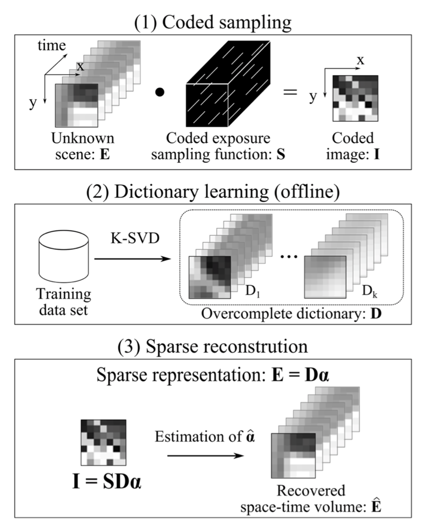
Denote the space-time volume corresponding to an $M\times M$ pixel neighborhood and one frame integration time of the camera as $E(x,y,t)$. A projection of this volume along the time dimension is captured by a camera. A $N$ times gain in temporal resolution needs to be achieved, i.e., recovery of space-time volume $E$ needs to be done at a resolution of $M\times M\times N$. Let $S(x, y, t)$ denote the per-pixel shutter function of the camera within the integration time $(S(x, y, t) \in {0,1} )$. Then, the captured image $I(x, y)$ is

Rewriting the above equation in the matrix form as $\textbf{I} = \textbf{S}\textbf{E}$. $\textbf{I}$ which is the vector of observations has a size $M^{2}$ and $\textbf{E}$ which is the vector of unknowns has a size $N \times M^{2}$. To solve the under-determined system of equations above, techniques of compressed sensing are used. The sytem above can be solved faithfully if the signal $\textbf{E}$ has a sparse representation $\boldsymbol{\alpha}$ in a dictionary $\textbf{D}$:

where $\boldsymbol{\alpha} = [\alpha_{1},\cdots,\alpha_{k}]^{T}$ are the coefficients, and $\textbf{D}_1, \cdots , \textbf{D}_k$ are the elements in dictionary $\textbf{D}$. The coefficient vector $\boldsymbol{\alpha}$ is sparse. The over-complete dictionary $\textbf{D}$ is learned from a random collection of videos. The space-time volume $\textbf{E}$ is sampled with a coded exposure function $\textbf{S}$ and then projected along the time dimension, resulting in a coded exposure image $\textbf{I}$.

An estimate of the coefficient vector $\hat{\boldsymbol{\alpha}}$ can be obtained by solving a standard problem in compressed sensing:

\begin{equation} \hat{\boldsymbol{\alpha}} = \arg \min_{\alpha} \lVert \alpha \rVert_{0} \text{ subject to } \lVert \textbf{S}\textbf{D}\boldsymbol{\alpha} - \textbf{I} \rVert_{2}^{2} < \varepsilon \end{equation}

The space-time volume is computed as $\hat{\textbf{E}} = \textbf{D}\hat{\boldsymbol{\alpha}}$. A pictorial representation of the approach containing three steps viz. coded sampling, dictionary learning and sparse reconstruction is given in figure below (taken directly from Hitomi et al.).

Sampling Strategies

Continuous Bump

The continuous bump sampling strategy is a strategy that satisfies hardware constraints and is proposed by Liu et al. It satisfies the following constraints:

• Binary shutter: The sampling function $\textbf{S}$ takes values in ${0,1 }$. At any time $t$, a pixel is either collecting light (1-on) or not (0-off).
• Single bump exposure: Each pixel can have only one continuous “on” time (i.e., a single bump) during a camera integration time.
• Fixed bump length: The bump length is fixed for all pixels.

We implement this strategy as follows: 1. For each pixel in the input video, the bump start time is selected uniformly randomly, i.e., the bump start time at any pixel can be $t$ with probability $1/N$ where $N$ is the temporal depth of $\textbf{E}$. 2. Space-time volume at a pixel is added when the shutter function is $1$. The coded image is constructed by averaging the above sum.

Random Sampling

In this sampling strategy, the bump period may not be continuous. Fix a bump length $b$ and let the temporal depth be $N$, then this strategy is implemented as follows: 1. For every point in an input video, i.e., a point described by $(x,y,t)$, the shutter function takes value 1 with probability $b/N$. 2. Space-time volume at a pixel is added when the shutter function is $1$. The coded image is constructed by averaging the above sum. It might happen for a pixel location that the number of time instants where shutter function takes value 1 is not equal to the bump length.

Distributed Bump

Here, we constrain that for every pixel location, the number of time instants where shutter function takes value 1 is equal to the bump length. This is implemented as follows: 1. Generate $b$ distinct random integers between $1$ and $N$. 2. Space-time volume at a pixel is added when the shutter function is $1$. The coded image is constructed by averaging the above sum.

Comments and Conclusions

For more information about OMP and K-SVD algorithm and details on our experimental setup and detailed results, I encourage the reader to see our report here. Finally, we have concluded that the method that we have experimented with, in this project, can reconstruct the videos with high temporal resolution without compromising on spatial resolution, though some artifacts are visible, most likely because of smaller dictionary size that we have used. We observed the effect of changing different hyper-parameters. We also observed that distributed bump sampling produces the best results, but this has to be at the cost of increased hardware complexity.

References

Video from a Single Coded Exposure Photograph using a Learned Over-Complete Dictionary
Yasunobu Hitomi, Jinwei Gu, Mohit Gupta, Tomoo Mitsunaga, Shree K. Nayar (2011)

Efficient Space-Time Sampling with Pixelwise Coded Exposure for High-Speed Imaging
Dengyu Liu, Jinwei Gu, Yasunobu Hitomi, Mohit Gupta, Tomoo Mitsunaga, Shree K. Nayar (2014)