Tutorial on Attention-based Models (Part 2)

19 minute read

Published: June 11, 2018

In part one of this series, I introduced the fundamentals of sequence-to-sequence models and attention-based models. I briefly mentioned two sequence-to-sequence models that don't use attention and then introduced soft-alignment based models. In this post, I’m going to discuss about various monotonic attention mechanisms.

3.2. Monotonic Alignments

Monotonic alignments are motivated by the limitations of soft alignments i.e. the quadratic-time complexity and no option for online decoding. The mechanisms discussed achieve quadratic-time training but linear-time decoding and the facility of online decoding as well.

3.2.1. Hard Monotonic Mechanism [paper]

Hard monotonic alignments attend to exactly one vector in memory $h_j$ at output time step $i$ i.e. $c_i = h_j$, unlike soft alignments which use expectation over complete memory to calculate the context vector.

If model attends to the input time step $t_{i-1}$ at the output time step $i-1$, we calculate the energy of $h_j$ where $j \in \{t_{i-1}, t_{i-1}+1, \ldots, T\}$ i.e. starting from the memory previously used. We pass each energy output through the logistic sigmoid function to produce 'selection probability' $p_{i, j}$ and sample $z_{i, j}$ from $Bernoulli(p_{i, j})$.

&&e_{i, j} = MonotonicEnergy(s_{i-1},h_j)&&

&&p_{i,j} = \sigma(e_{i,j})&&

&&z_{i,j} = Bernoulli(p_{i,j})&&

As soon as we see $z_{i, t_i} = 1$, we stop and use $h_{t_i}$ as our context vector and repeat the above process starting from input time step $t_i$ at output time step $i$. If $z_{i, j} = 0~\forall~j\in\{t_{i-1}, t_{i-1}+1, \ldots, T\}$, we set $c_i = \mathbf{0}$.

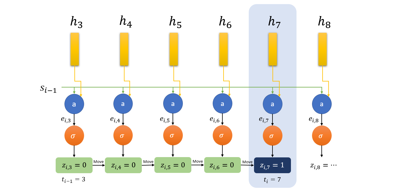Here is an example of output time step of hard monotonic mecchanism. Here $t_{i-1} = 3$ is the index of memory vector selected at previous step. Model, therefore, starts from $h_3$ and moves forward until it finds $z_{i,7}=1$. Hence, $h_7$ is selected as $c_i$ and we say that $t_i=7$.

Note that the above model only needs $h_k, k\in\{1, 2, \ldots,j\}$ to compute $h_j$. If we use a unidirectional RNN as the encoder, we can perform online decoding where the time complexity will be $\mathcal{O}(\max\{T, U\})$. Also note that, because of sampling, we cannot train this model using back-propagation. We, therefore, use the expectation of $h_j$ during training (inspired from soft alignments) and try to induce discreteness into $p_{i,j}$ to later decode monotonically. The $\alpha_{i,j}$ defines the probability that input time step $j$ is attended at output time step $i$. We go through a simple, worded derivation below for the calculation of $\alpha_{i,j}$. (You can skip it in the first pass of reading.)

&&\alpha_{i, j} = \mathbb{P}_i(h_j\text{ used}) = \mathbb{P}_i(h_j\text{ used}|h_j\text{ checked})\mathbb{P}_i(h_j\text{ checked})&&

&&\mathbb{P}_i(h_j\text{ used}|h_j\text{ checked}) = p_{i,j}&&

&&\mathbb{P}_i(h_j\text{ checked}) = \mathbb{P}_i(h_{j-1}\text{ not used}, h_{j-1}\text{ checked}) + \mathbb{P}_{i-1}(h_j\text{ used}|j\text{ checked})&&

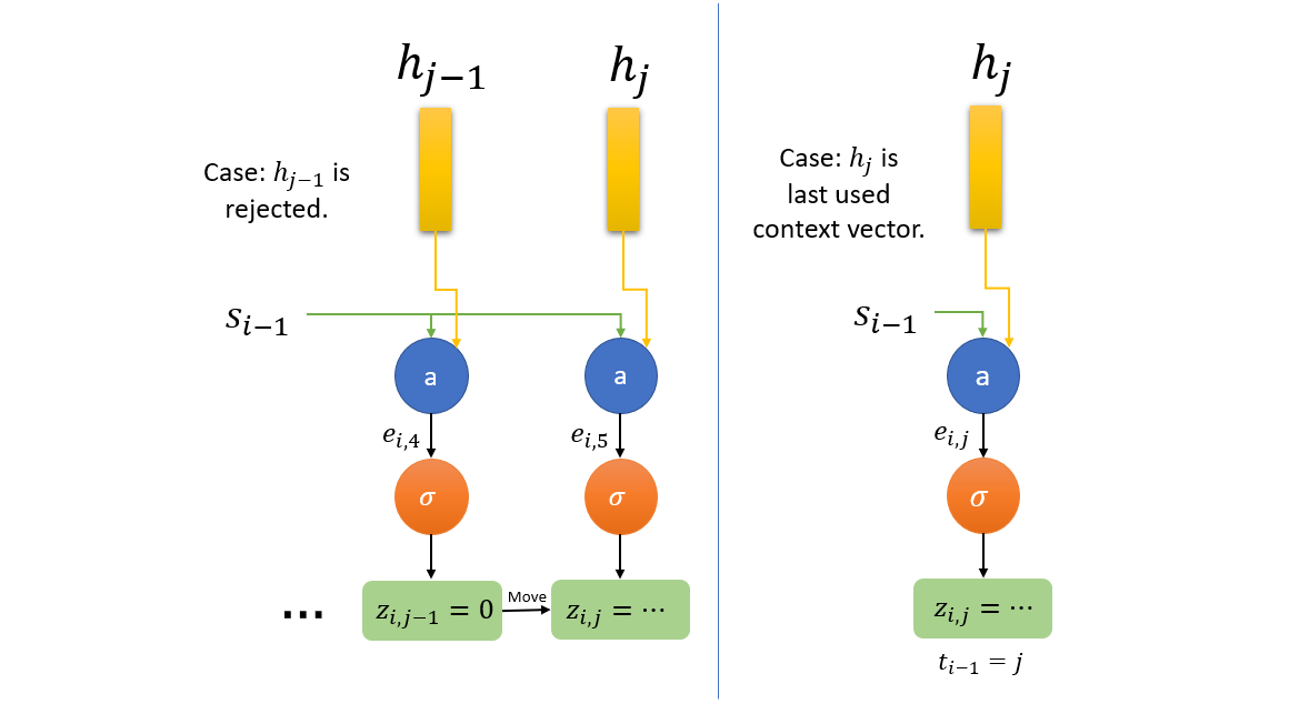Two possible cases are depicted when $h_j$ is a candidate for context vector. First case on left: $h_j$ is candidate because $h_{j-1}$ was rejected i.e. $z_{i,j-1}=0$. Second case on right: model starts from $h_j$ itself as it was the last used context vector i.e. $c_{i-1}=h_j$ or $t_{i-1} = j$.

The last relation can be reasoned out by noting that $h_j$ will be a candidate for context vector either when $h_{j-1}$ is rejected or $h_j$ itself was selected as context vector in previous output time step $i-1$. Using above relations for memory vector $h_{j-1}$, we get the relations

&&\mathbb{P}_i(j-1\text{ checked}) = \frac{\alpha_{i,j-1}}{p_{i,j-1}}&& &&\mathbb{P}_i(j-1\text{ not used}|j-1\text{ checked}) = 1-p_{i,j-1}&&

Finally putting all relations together, we get

&&\alpha_{i,j} = p_{i,j} \Big((1-p_{i,j-1})\frac{\alpha_{i,j-1}}{p_{i,j-1}} + \alpha_{i-1,j}\Big)&&

which can also be written as following, allowing us to compute this parallelly by writing it in terms of cumulative products and cumulative sums.

&&q_{i,j} = \frac{\alpha_{i,j}}{p_{i,j}} = (1-p_{i,j-1})q_{i,j-1} + \alpha_{i-1,j}&&

A tricky way to promote discreteness, a zero-mean unit-variance Gaussian noise is added to logistic sigmoid activation. This forces the model to learn to produce $p_{i,j}$ close to zero or one, effectively making it binary.

Energy function used for hard monotonic alignments is as follows:

&&\text{MonotonicEnergy}(s_{i-1},h_j) = g\frac{v^T}{||v||}\tanh(W_s s_{i-w}+W_h h_j+b)+r&&

It is very similar to Bahdanau energy function but a little different because sigmoid function applied on monotonic energy is not shift-invariant like the softmax function. Therefore, for giving in more control on values of energy, the vector $v$ in Bahdanau energy is replaced by a normalized vector $\frac{v}{||v||}$ and then scaled with a scalar $g$ and offset with a scalar $r$. As you might guess, $g$ and $r$ are also learned parameters.

3.2.2. Monotonic Chunkwise Mechanism [paper]

Hard monotonic alignments which I just described are just too hard in their conditions! Using only one vector $h_{t_i}$ as context vector $c_i$ is a little too much constraint and this is reflected in its poor performance on some tasks. A novel solution to this problem is Monotonic Chunkwise Mechanism.

We use a middle path between soft alignments and hard monotonic alignments by allowing the model to use soft attention over fixed-size chunks (say, size $w$) of memory ending at input time step $t_i$ for each output time step $i$. Therefore, model uses a context vector derived from memory elements ${h_{v}, h_{v+1}, \ldots h_{t_i}}$ where $v= t_i-w+1$. The memory index $t_i$ is derived in the same way as in the hard monotonic mechanism. The energy of each memory element is given by the following equation.

&&u_{i,k} = \text{ChunkEnergy}(s_{i-1}, h_k) = v^T \tanh(W_{s}s_{i-1} + W_{h}h_j + b)&&

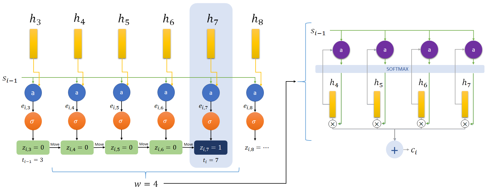A diagram showing the flow of monotonic chunkwise mechanism. Notice that a soft alignment over a chunk of size $w=4$ is applied in addition to monotonic attention. First, using mechanism explained in an earlier figure, $h_7$ is selected. Then a soft alignment is used over a chunk ending at $h_7$.

The context vector is given by a weighted sum of $w$ memory elements ending at $t_i$. This is exactly applying soft-alignment over small chunks!

&&c_i = \sum_{k=v}^{t_i}\frac{\exp(u_{i,k})}{\sum_{l=v}^{t_i}\exp(u_{i,l})}h_k&&

Similar to the training in the hard monotonic mechanism, we need to take expected value of context vector by using the induced probability distribution. We use the $\alpha_{i,j}$ derived for the hard monotonic mechanism. Given below is (another!) worded derivation of $\beta_{i,j}$ which is the probability of using $h_j$ as context vector for output time step $i$.

&&\beta_{i,j}=\mathbb{P}_i(h_j\text{ used}) = \sum_{k=j}^{j+w-1}\mathbb{P}_i(h_j\text{ used}|t_i = k)\mathbb{P}(t_i = k)&&

&&\mathbb{P}_i(h_j\text{ used}|t_i = k) = \frac{\exp(u_{i,k})}{\sum_{l=v}^{t_i}(u_{i,l})}&&

&&\mathbb{P}(t_i = k) = \alpha_{i,k}&&

&&\beta_{i,j}=\sum_{k=j}^{j+w-1} \frac{\exp(u_{i,k})}{\sum_{l=v}^{t_i}\exp(u_{i,l})}\alpha_{i,k}&&

The equation derived for $\beta_{i,j}$ can be parallelized using moving sum and computation, therefore, is very efficient. Note that number of parameters have increased (and therefore computations as well) as monotonic chunkwise mechanism is using both $\text{MonotonicEnergy}(s_{i-1}, h_j)$ and $\text{ChunkEnergy}(s_{i-1}, h_j)$. This increase is very marginal, about $1\%$, but the performance of model increases significantly, reaching almost at par with soft alignments for some tasks.

3.2.3. Limitations of Monotonic Alignments

There are two major limitations of the hard monotonic mechanism. First, the one we discussed as a motivation for the chunkwise monotonic mechanism, is that there is not enough context in the context vector as we force the model to capture complex dependencies only using a single memory vector. This concern is almost resolved by using chunks of memory summed over a soft distribution.

The second limitation is the assumption of strict monotonicity in input and output alignments. For example, in translation task, we can expect a degraded performance when translation is performed on languages with different sentence structure i.e. a different order of subject, verb and object, though this assumption can be almost true for structurally similar languages.

We note here that soft alignments, though computationally expensive and unsuited for online decoding, are robust to input-output alignment relations and use a much wider context for producing outputs as compared to monotonic alignments.

References

Online and Linear-Time Attention by Enforcing Monotonic Alignments
Colin Raffel, Minh-Thang Luong, Peter J. Liu, Ron J. Weiss, Douglas Eck
Proceedings of the 34th International Conference on Machine Learning, 2017

Monotonic Chunkwise Attention
Chung-Cheng Chiu, Colin Raffel
International Conference on Learning Representations, 2018

Tutorial on Attention-based Models (Part 2)

3.2. Monotonic Alignments

References

Further Reading

Share on

Leave a Comment

You May Also Enjoy

How to Undergrad

An Introduction to Multi-Armed Bandits and Markov Decison Processes

Batch Arm Pulls for Stochastic Multi-Armed Bandits

Voice Conversion using GANs: An Extensive Review