Tutorial on Attention-based Models (Part 1)

37 minute read

Published: June 02, 2018

Teaser: The task of learning sequential input-output relations is fundamental to machine learning and is especially of great interest when the input and output sequences have different lengths. Applications such as speech recognition, machine translation, document summarization, image captioning and many more can be posed in this format. In this post, we explore one of the popular ways to solve such problems using 'Attention Based Models'.

1. Introduction

The task of learning sequential input-output relations is fundamental to machine learning and is especially of great interest when the input and output sequences have different lengths. Applications such as speech recognition, machine translation, document summarization, image captioning and many more can be posed in this format. There was no satisfactory framework in deep learning for solving such problems for quite some time until recently when researchers in deep learning came up with some, well.., new ideas. We explore one of the popular ways to solve such problems using 'Attention Based Models'. If you're completely new to this idea, this post will serve as a starting point. I assume a basic background in neural networks (multilayer and bi-directional recurrent NNs) and basics of probability. For the familiar ones, you might be helped by some new thoughts and some new variations or simply use it as a refresher.

One of earlier ways to solve such problems, as we shall discuss later, was to compress a sequential input into a fixed size vector and this vector was fed to a recurrent neural network (RNN) to generate a sequence of outputs. Attention-based models, on the other hand, set us free to use variable-length inputs without the compulsion of compressing them down to a fixed-size vector by using a variable-length memory. Model is free to use this memory in a very flexible manner to generate the output sequence. Moreover, different parts of memory can be accessed at different output time steps. These models are well-motivated because information is lost by compressing long variable-length sequences into a fixed-size vector and deciding (or learning!) the compression is an additional task to solve.

2. Basic Structure of Attention-Based Model

2.1. Sequence-to-sequence models

Attention-based models belong to a class of models commonly called sequence-to-sequence models. The aim of these models, as name suggests, it to produce an output sequence given an input sequence which are, in general, of different lengths. Let input sequence be $\mathbf{x} = \{x_1, x_2, \ldots, x_T\}$ and output sequence be $\mathbf{y} = \{y_1, y_2, \ldots, y_U\}$. There are 2 parts of a sequence-to-sequence models viz. encoder and decoder, both of which are RNNs. Encoder encodes the given input producing a series of hidden states $\mathbf{h} = \{h_1, h_2, \ldots, h_T\}$ of input $\mathbf{x}$.

Because of sub-sampling (which is common), the length of hidden state sequence can be less than the length of input sequence. For example, sub-sampling by 2 at each layer of a 3-layered RNN will decrease the hidden state sequence length by a factor of 8. For clarity in this article, we assume that there is no sub-sampling.

&&\mathbf{h} = Encoder(\mathbf{x})&&

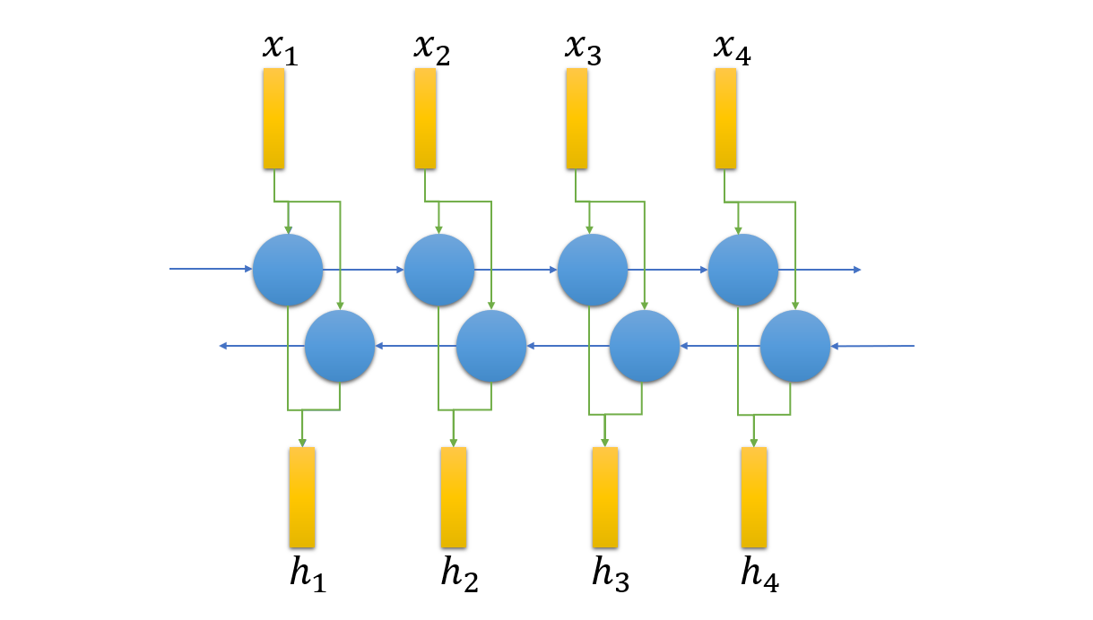Bi-directional RNN based encoder takes the input sequence $\mathbf{x} = \{x_1, x_2, \ldots, x_T\}$ outputs the hidden states $\mathbf{h} = \{h_1, h_2, \ldots, h_T\}$ (memory vectors).

These hidden states are also collectively referred to as 'memory'. Decoder part can use this memory in different ways to produce output sequence $\mathbf{y}$. A common way is to first convert this memory into context vectors $c_i$ for each output time step $i={1, 2, \ldots, U}$. We will soon focus on how to create these context vectors. For each output time step, the output $y_i$ of decoder RNN depends on $c_i$ and $s_i$ where $s_i$ is the state of the decoder RNN. Decoder state further depends on context vector at present time step $c_i$, output at previous time step $y_{i-1}$ and previous state $s_{i-1}$.

Note: Even if you feel lost at this point because of notation, go on reading further as I explain the model in much greater detail. Remember that we have an input sequence $\mathbf{x}$ and a hidden state sequence $\mathbf{h}$ of length $T$ and an output sequence $\mathbf{y}$ of length $U$. All the hidden states of the encoder RNN are contained in $\mathbf{h}$ and the decoder RNN state is denoted by $s_i$ at output time step $i$. It should be noted that the encoder and decoder RNN time steps are treated very independently as input sequence is now encoded to form a memory made up of vectors $\mathbf{h} = \{h_1, h_2, \ldots, h_T\}$ and output sequence generation is the major focus of the remaining article. One can think of the context vector as the information used to generate the output. Each output in the output sequence requires a new context and some information from the past!

&&s_i = Decoder(c_i, y_{i-1}, s_{i-1})&&

&&y_i = OutputFunction(s_i, c_i)&&

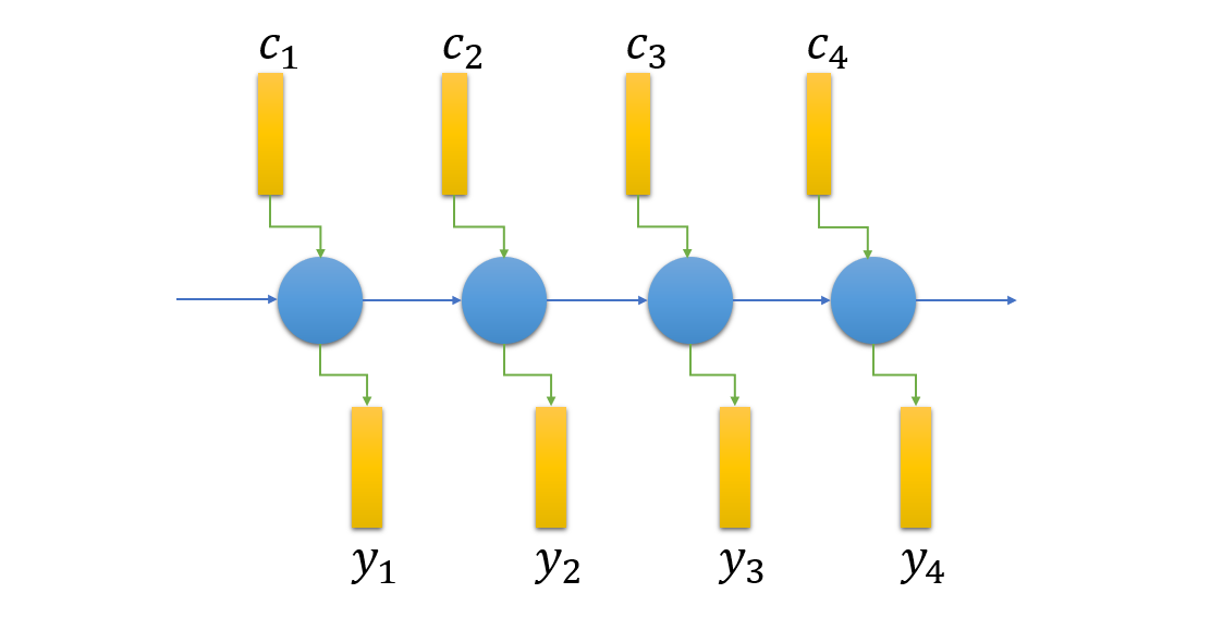At each decoder output step $i$, inputs to the RNN cell are $c_i$, $y_{i-1}$ and $s_{i-1}$ and outputs the vectors $s_{i}$ and $y_i$. First step takes input start-of-sequence flag <s>.

2.2. Attention-Based Models

[paper]

Attention-based models describe one particular way in which memory $\mathbf{h}$ can be used to derive context vectors $c_1, c_2, \ldots, c_U$. Putting it simply, attention-based models have the flexibility to look at all these vectors $h_1, h_2, \ldots, h_T$ i.e. memory and decide which one is to be used as the context vector that is fed to the decoder RNN at each output time step. If $h_j$ is being used as $c_i$, we say that model is paying attention (or simply, attending) to $j^{th}$ vector in memory at output time step $i$. We will soon see what all mechanisms can be used to look at memory to decide context vectors.

2.2.1 Encoder

The encoder part is generally a multi-layered bi-directional RNN made of LSTM or GRU cells. In some cases, uni-directional RNNs have also been used to process input from left to right. In particular, online decoding requires uni-directional RNN as the complete input sequence is not available for fast decoding. When the encoder is bi-directional, vectors $h_1, h_2, \ldots, h_T$ are formed by concatenation of outputs from forward and backward cells.

2.2.2. Decoder

The decoder is generally a multi-layered uni-directional RNN made of LSTM or GRU cells and an output layer/function. As stated earlier, $s_i$ denotes the state of this RNN. Decoder, at each output time step, uses previous output $y_{i-1}$ and context vector $c_i$ in addition to its previous state $s_{i-1}$. Output function uses current decoder state $s_i$ and context vector $c_i$ to produce output $y_i$. For example, this function can be a trainable softmax layer if the output is categorical.

2.3. Background: Models Without Using Attention

Before we go on to discuss the various attention mechanisms, we start with sequence-to-sequence models that don't use attention. We aim to get an idea of developments before attention-based models and how these models are less flexible in their choice of context vectors.

2.3.1 Using Two Deep-LSTM Networks [paper]

In this model, we use two deep unidirectional LSTM networks each of 4 layers. First LSTM network reads the input and generates a fixed-dimensional vector, an encoding, which contains the summary of the complete input. This summary is then fed to the second LSTM, the decoder, which generates the output vectors. We can think of this network in the framework we earlier developed by using the following equation.

&&c_i = h_T&&

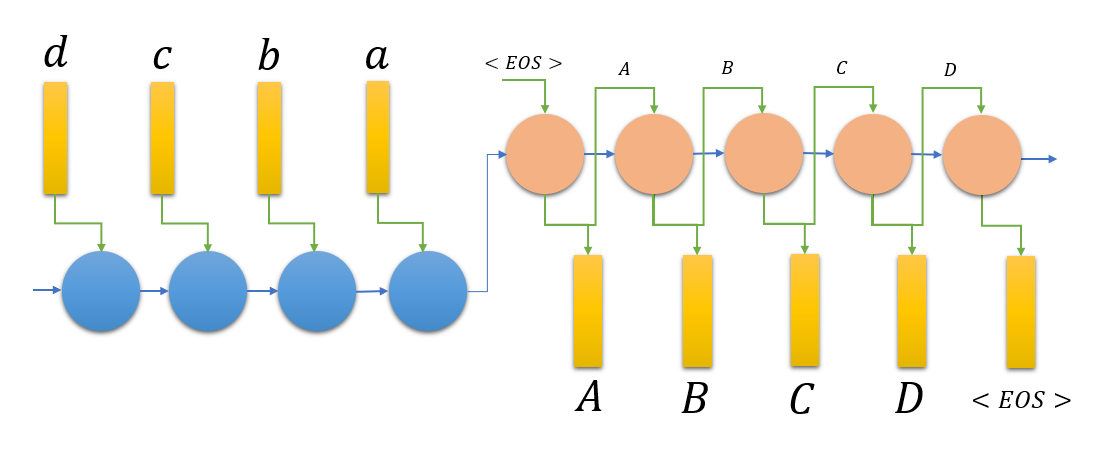The input sequence can be, for instance, words (for translation task) in the source language and an end-of-sentence (<EOS>) tag at its end. The output generated is a sequence of words in the target language and it ends when the tag is generated by decoder LSTM network. A major problem with this network is the long-range dependencies that it introduces between relevant pairs of input and output network. A clean trick is to reverse the input sequence to make short-term dependencies between initial sequence and it has been shown that it improves performance by a significant amount.

Two LSTM networks are being used where first input LSTM takes the complete input sequence and outputs the 'summary' vector $h_T$ which is fed to the decoder LSTM.

As compared to a single-LSTM-based network where it both reads and generates input and output respectively, this network has more parameters and it can, therefore, learn more complex relations. For translation task example we considered above, intuitively, the two LSTM networks are learning 2 different languages and a message is passed on from the first network to second network using the summary vector. This summary vector, intuitively speaking, contains content-information in some universal language which both LSTM networks understand.

2.3.2 Bi-directional LSTMs with Connectionist Temporal Classification [paper]

If the length of the output sequence is at most equal to the length of the input sequence, we can use single RNN such as a bi-directional LSTM which produces outputs for each input time step. Since the number of outputs produced will be more than the actual number of outputs, we introduce a 'blank' flag which is interpreted as no output produced. Further, the inference is done by removing all the 'blank' flags and contiguous repeated outputs.

For example, both the output sequences 'a - a a b - b b' and 'a a - - a b - b' mean the same sequence 'aabb' (- is the 'blank' flag).

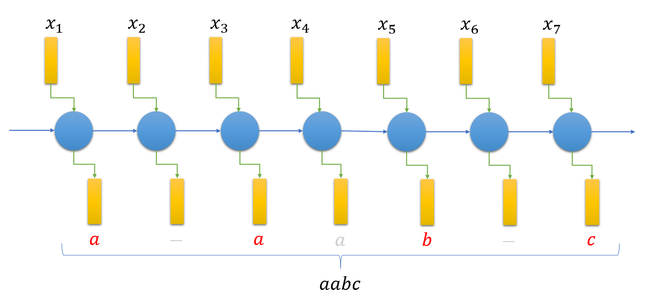A RNN (like bi-directional LSTM) is used to generate output sequence from which repeated outputs and blanks are removed for inference.

The most interesting thing about CTC model is the way training objective is defined and used. I don't go into the details of the objective function in this article but it is sufficient here to say that the objective function computation and training are efficiently done by the forward-backward algorithm.

3. Attention Mechanisms

3.1. Soft Alignments

[paper]

We started to think of $c_i$ as one of the vectors among those available in memory $\mathbf{h}$. An attention mechanism is free to choose one vector from this memory at each output time step and that vector is used as context vector. As you might have guessed already, an attention mechanism assigns a probability to each vector in memory and context vector is the vector that has the maximum probability assigned to it.

&&e_{i,j} = a(s_{i-1}, h_j)&&

&&\alpha_{i,j} = \mathbb{P}_i(h_{j}) = softmax(e_{i,:})_j&&

&&c_i = h_{\arg \max_{j} \alpha_{i,j}}&&

Here $e_{i,j}$ is the energy function for calculating unnormalized scalar energy of each vector $h_j$ in memory given the previous decoder state $s_{i-1}$. We can think of this function as the 'decision-maker' who looks at the state of decoder and decides the eligibility of all memory vectors to become context vector. Using softmax function, we normalize all $e_{i,j}$ to obtain the probability distribution $\mathbf{\alpha}_i = {\alpha_{i, 1}, \alpha_{i, 2}, \ldots, \alpha_{i, T}}$.

The model described above is not used directly though. The probability distribution assigned to vectors in memory can be fairly non-peaky i.e. not favouring a particular vector, especially during the initial part of the training. This suggests that we should sample from this distribution and use an averaged context vector i.e. simply the expectation of $h_j$ over distribution $\mathbf{\alpha}_i$.

&&c_i = \sum_{j} \alpha_{i, j} h_j&&

Because $\alpha_{i,j}$ is weight of each element in memory, we call the distribution $\mathbf{\alpha}_{i}$ as 'alignment' of the memory at output time step $i$. The vector $c_i$ is also referred to as 'attention' when talking about attention mechanisms. Also, note that we named this section of attention mechanisms as soft alignments because we are not just using one vector from memory but a linear combination of these vectors.

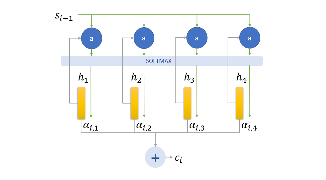Previous decoder RNN state $s_{i-1}$ is mixed with every memory vector to get energy corresponding to the memory and softmax over these energies is used to get the alignment probabilities.

In the following two soft alignment mechanisms viz. Luong Mechanism and Bahdanau Mechanism, the major difference is the calculation of the energy of each vector in memory i.e the function $a(s_{i-1}, h_j)$.

3.1.1. Luong Mechanism [paper]

Luong Mechanism calculates the energy by taking the dot product of $s_{i-1}$ with each vector $h_j$ in memory.

&&a(s_{i-1}, h_j) = s_{i-1}\cdot h_j&&

If the size of the state vector and memory vectors are not equal, a dense layer can be applied to one of them to ensure that dot product exists. Also, note that the number of parameters in Luong energy function is zero which is in contrast with Bahdanau mechanism. Though the two papers have a lot of differences, I mainly borrow this naming from TensorFlow library.

3.1.2. Bahdanau Mechanism [paper]

Bahdanau Mechanism uses a fully connected layer on $s_{i-1}$ and $h_j$ and also brings them to the same dimension as a result. It applies a hyperbolic tangent layer to the sum of the outputs of these fully connected layers. One can simply think of this function as a flexible mixer of encoder state and memory vector.

&&a(s_{i-1}, h_j) = v^T \tanh(W_{s}s_{i-1} + W_{h}h_j + b)&&

Luong Mechanism, as mentioned above, has an unparameterized energy function whereas Bahdanau Mechanism uses a parameterized energy function. Since the dot product is maximum when the two vectors are equal, Luong Mechanism puts a harsh condition on state vector to be directed along the desired context vector and orthogonal to other vectors in memory. Bahdanau Mechanism, on the other hand, is much more flexible and performs at par with or better than Luong Mechanism.

3.1.3. Viewing Attention

Alignment of memory gives us a door to look into how the model is working as it produces the output. Higher probability assigned to a memory element is associated with its high importance in generating the output. In machine translation task, for example, we expect a high probability assigned to input word whose translated word is being generated. An example is shown for clarity.

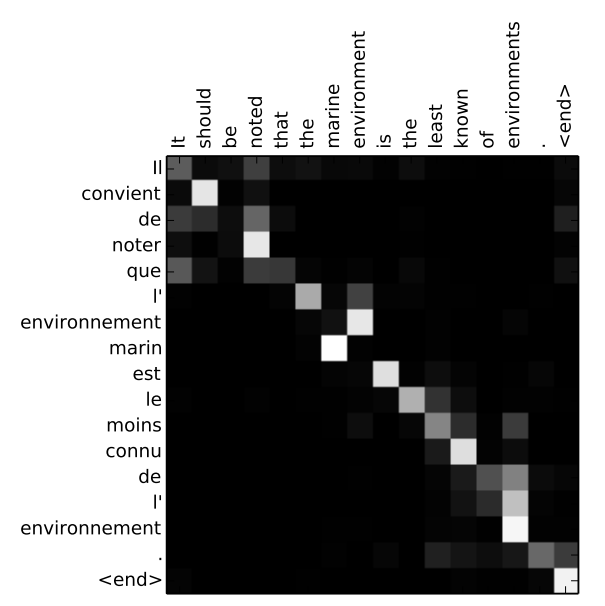A visualization of how the model is paying attention to various parts of input sequence while producing outputs. The brighter is the square, higher is the probability assigned to that memory vector.

If you want to read about Neural Turing Machines and other cool models and play with visualizations, see this very interesting post Attention and Augmented Recurrent Neural Networks by Olah and Carter on Distill.

3.1.4. Limitations of Soft Alignments

There are two major limitations of soft alignments. First is the quadratic time complexity which is evident as attention score is computed for every vector in memory at every output time step, resulting in time complexity of $\mathcal{O}(TU)$. The second limitation is that soft alignment mechanisms need all inputs before the first output can be computed which makes this model unsuited for online applications. We, therefore, aim to reduce the time complexity of the attention-based models and intelligent use of inputs for online decoding.

I'll be adding a part 2 of this series of posts soon. In the second part, I mostly intend to discuss how monotonic attention and hard alignment are attempts to eliminate the limitations of soft-alignment based models. Please send any suggestions, comments or corrections to my email given at the bottom of the page or add an issue on my repository here.

Update: Link to Part 2.

References

Learning Phrase Representations using RNN Encoder-Decoder for Statistical Machine Translation
Kyunghyun Cho, Bart van Merrienboer, Caglar Gulcehre, Dzmitry Bahdanau, Fethi Bougares, Holger Schwenk, Yoshua Bengio
Proceedings of the 2014 Conference on Empirical Methods in Natural Language Processing (EMNLP)

Sequence to Sequence Learning with Neural Networks
Ilya Sutskever, Oriol Vinyals, Quoc V. Le
Proceedings of the 27th International Conference on Neural Information Processing Systems (NIPS 2014)

Connectionist Temporal Classification: Labelling Unsegmented Sequence Data with Recurrent Neural Networks
Alex Graves, Santiago Feránandez, Faustino Gomez, Jürgen Schmidhuber
Proceedings of the 23rd International Machine Learning Conference, 2006

Neural Machine Translation by Jointly Learning to Align and Translate
Dzmitry Bahdanau, Kyunghyun Cho, Yoshua Bengio
International Conference on Learning Representations, 2015

Effective Approaches to Attention-based Neural Machine Translation
Minh-Thang Luong, Hieu Pham, Christopher D. Manning Proceedings of the 2015 Conference on Empirical Methods in Natural Language Processing

Addtional Notes

In section 2.3.1, the architecture uses 4-layered LSTM model for both input-sequence reading and generating output-sequence. Long-range dependencies refer to the temporal dependencies in sequences and not the forward pass of the model.
In section 2.3.1, suppose an input sequence $a-b-c-d$ has to be translated to output sequence $A-B-C-D$. If input LSTM model sees $d-c-b-a$ instead of $a-b-c-d$, the output 'summary' vector is influenced most by $a$ and hence it becomes easier to realize for output LSTM to start with $A$. Although average dependency length between the pairs ($a-b-c-d$, $A-B-C-D$) and ($d-c-b-a$, $A-B-C-D$) is same, the model probably finds it easier to start the sequence with initial $A$ and $B$ and so on. Temporal dependencies later help in generating the $C$ and $D$ more easily on average. This is very crude reasoning and there is no 'proof' as such but this phenomenon of better performance on the input sequence reversal is observed and can be explained as above.

Share on

Twitter Facebook LinkedIn

Tutorial on Attention-based Models (Part 1)

1. Introduction

2. Basic Structure of Attention-Based Model

2.1. Sequence-to-sequence models

2.2. Attention-Based Models

2.3. Background: Models Without Using Attention

3. Attention Mechanisms

3.1. Soft Alignments

References

Further Reading

Addtional Notes

Share on

Leave a Comment

You May Also Enjoy

How to Undergrad

An Introduction to Multi-Armed Bandits and Markov Decison Processes

Batch Arm Pulls for Stochastic Multi-Armed Bandits

Voice Conversion using GANs: An Extensive Review